Doubt on Running Casing

Recently I was put in a new job, in a new way of life ... my life was put up-side down. Now I need to relearn spanish and learn to work in the office. Quite nice in fact.

While performing a monitoring job in a deep-water well, I had one of my colleagues asking me why the casing we were running was behaving in a funny way.

The funny way she was meaning, was a reduction at the hook-load reading while running it into the bottom of the well.

Next post I will answer this.

Watching the World Cup Opening with my colleagues in Ciudad del Carmen.

Taking a walk and bad pictures in Ciudad del Carmen.

Jet Nozzle Flow and CFD Simulation

2 Jet Nozzle Flow

2.1 Hydraulic Impact Force

In the drilling industry we usually assume that the jet will impact the hole bottom without loss of momentum [7] and, sometimes, can be wrongly interpreted (mainly when we have a big clearance between the bit attack area and the bottom of the well) as having the same velocity profile hitting the bottom. Lets us take the most used formula to calculate the hydraulic impact force in pounds:

(1) F_j = 0.01823C_dq√(ρΔp_b)

Where C_dis a discharge coefficient that ranges between 0.95 and 1.03; q is the flow rate in gpm; ρ, the fluid density in pounds per gallon and Δp_bis pressure drop across the bit in psi. Having this in mind and taking into consideration an usual drilling parameters regarding hydraulics we have the following:

TFA	Cd	q	ρ	Δpb	Fj
0.969 in²	0.95	600 gpm	9.6 ppg	338.9 psi	592.7 lbf
625.16 mm²	0.95	2271.25 lpm	1.15 g/cm³	2.3366 MPa	2636.46 N

Proceeding with a simple math, following the assumption that the jet won’t spread out before hitting the bottom and every jet (doesn’t matter its diameter) will keep the same impinging velocity, we have a hydraulic impact pressure value of 611 psi ( 4.2127 MPa ) for each nozzle.

2.2 Spreading Out the Jet and Cavitating Clouds

It is going to be seen that the flow of submerged jets are well known [8] and posses some distinct regions (4↓):

Figure 4 The flow regions of an impinging jet (adapted from Zuckerman)[8].

From (4↑) is possible to see that when the jet exits the nozzle, the velocity gradient creates shearing at the edges which transfers momentum. Taking into account this process we can easily visualize the jet dissipates energy and the velocity profile is widened.

Sato et al [9] carried out experiments where they had a submerged jet nozzle and they used these experiments to investigate the occurrence of cavitating clouds where they saw a ring-like erosion distribution over an acrylic plate that could be related to cavitation on impinging walls. Hutli [10]concluded through experiments that the cavitation exhibits a regular frequency of oscillation. It is known that cavitation in a well can occur on very shallow depths, but when we are deep is quite difficult its appearance. The key behind bringing this subject is the already mentioned statement "cavitation exhibits a regular frequency of oscillation", so, if cavitation happens on submerged nozzles in above mentioned experiments, the occurrence of low pressure zones in deep wells are possible and they are cyclic.

3 CFD Simulation

Having this background, and in order to capture these low pressure zones, were simulated the same boundary geometry (5↓) and three different nozzle diameters having a high density of nodes at the shear layer: 10/32" (7↓), 12/32" (8↓) and 14/32" (9↓) with 60 m/s (196.85 ft/s) of jet velocity with the same drilling fluid parameters ( MW= 9.6 ppg, YP= 27 cP, PV=22cP). The difference of hidrostactic pressure between the inlet of the nozzle and the bottom of the hole is negligible when compared with the impinging pressure.

The simulation was carried out using Openfoam on a Debian based computer with a transient PISO algorithm. Each run took 24 hours to be solved.

Figure 5 Simulation’s geometry.

Figure 6 20 degrees wedge simulation’s axisymmetric mesh. The flow is towards z-axis positive direction and the nozzle’s center is located at the origin .

We can see that the jet velocity (7↓,8↓,9↓), just before hitting the bottom of the well, is no longer the same as the nozzle exit and just at the impingement area we can see a stagnation region.

Figure 7 Velocity profile for 10/32" Nozzle with average exit velocity of 60 m/s (196.85 ft/s) after reaching fully developed flow.

Figure 8 Velocity profile for 12/32" Nozzle with average exit velocity of 60 m/s (196.85 ft/s) after reaching fully developed flow.

Figure 9 Velocity profile for 14/32" Nozzle with average exit velocity of 60 m/s (196.85 ft/s) after reaching fully developed flow.

The simulations regarding the pressure profiles gave us some very good results. The PISO algorithm uses the kinematic viscosity to solve the Navier Stokes equations, so, the results are the rho-normalized pressure with units in (m²/s²). For the case of this used drilling fluid we should expect values close to 2031 m²/s². We can see in ( 10↓, 11↓, 12↓ ) that the values are quite close to the expected value. In fact they are smaller, this is because in the F_j equation is not assumed we have energy losses between the jet and the surrounding fluid.

Figure 10 Pressure profile for 10/32" Nozzle. Maximum pressure of 1719 m²/s² (517 psi) and Minimum pressure of -510 m²/s² (-153 psi).

Figure 11 Pressure profile for 12/32" Nozzle. Maximum pressure of 1813 m²/s² (545 psi) and Minimum pressure of -606 m²/s² (-182 psi).

Figure 12 Pressure profile for 14/32" Nozzle. Maximum pressure of 1860 m²/s² (560 psi) and Minimum pressure of -1161 m²/s² (-349 psi).

References

[1] Carlos H.L. Bruhn, José Adilson T. Gomes, Cesar Del Lucchese Jr., and Paulo R.S Johann – “Campos Basin: Reservoir Characterization and Management – Historical Overview and Future Challenges”, OTC 15220, 2003.

[2] Bernardo, R.J, Saliés, J.B., and Polilo Filho, A.: “Campos Basin: Lessons Learned and Critical Issues to be Overcome in Drilling and Completion Operations”, OTC 15221, 2003.

[3] B. S. McLaury, S. A. Shirazi, Q. H. Mazumder, V. Viswanathan – “Effect of Upstream Pipe Orientation on Erosion in Bends for Annular Flow”

[4] Bill Chemerinski, SPE , Imperial Oil Resources, Ltd. and Leon Robinson, SPE, OGCI – “Hydraulic Wellbore Erosion While Drilling”

[5] Zeidler. H. Udo, Oyez Business Seminar, Innovations in Bit Technology, Oct. 9.1981, Houston. Texas – “Hydraulics and Hole Erosion”

[6] Steve Barton, Kirk Card, and Garrett Pierce, NOV Downhole – “Delivering Steering Success in Problematic Soft Formation Directional Wells”

[7] A. T. Burgoyne Jr., K. K. Milheim, M. E. Chevernet, F.S. Young Jr. - "Applied Drilling Engineering"

[8] N. Zuckerman and N. Lior - "Jet Impingement Heat Transfer: Physics, Correlations, and Numerical Modeling"

[9] K. Sato, Y. Sugimoto and S.Ohjimi - "Pressure-Wave Formation and Collapses of Cavitation Clouds Impinging on Solid Wall in a Submerged Water Jet"

[10] E. A. F. Hutli and M. S. Nedeljkovic - "Investigation of a Submerged Cavitating Jet Behavior: Part One - The Phenomenon, Detection Technique and Sono-Luminescence"

Jet Nozzle - Not well explained due to confidentiality

Again, it has been a while since my last post. But I reached a point with Openfoam that I don't know if it is confidential or not. Most of my simulations are taking into consideration of what I'm really observing at the field. One of the examples regards the jet impingement. This job is part of a bigger one where we have a jet flow from a bit nozzle hitting a wall.

Invest in Openfoam

It has been a while since my last post. This was caused by a project inside Schlumberger that took me away 3 months from Openfoam.

This was good because was a quite challenging job and made me value a lot my field job. In the meantime, I bought 2 Xeon CPU's and some other computer parts. Now ... I have a "biffy" computer to run my simulations 20 threads of processing power. Compared to my previous computer, this is a lot. ahhahaahaha


The only issue regarding these two CPUs is because I had to buy a Supermicro motherboard ... it is an EATX form factor (quite big) and here in Brazil we don't have such type of EATX case ... so ... I need to build one.

Right now my Frankenstein looks like this:

Quite ugly. But it is powerful and well cooled. hahahahahahah

I hope I find a way to build this EATX case.

Cheers!!!

Drill Pipe Rotation Influence

8 1/2" Well with 5 1/2" FH DP and 7" TJ - 60 RPM

8 1/2" Well with 5 1/2" FH DP and 7" TJ - 100 RPM

8 1/2" Well with 5 1/2" FH DP and 7" TJ - 160 RPM

8 1/2" Well with 5 1/2" FH DP and 7" TJ - No RPM

Merging Meshes from Salomé to be Used on Openfoam

This post took me a while. The main problem in here is due to mesh conversion between Salomé and Openfoam. Depending on your geometry, when you convert Salomé's unv file to Openfoam it appear some inner parts that are pretty annoying to get rid off.

If the mesh is pure unstructured you can do it easily. Just create and export. But if you have some structured mesh within a mesh, these inner parts come to play. One of my goals is to observe the velocity profile behavior and if you have an unstructured grid this won't be good, mainly because you won't have an even spaced velocity vector.

So, because of this issue, I had to redesign my straight stabilizer in order to have a hybrid grid. I had divided him into three main meshes and he is going to follow basically the same divisions stated at http://chasingaftermystuff.blogspot.com/2013/04/creating-spiral-drilling-stabilizer_12.html.

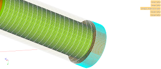
Follows the mesh from inner wall:

Zooming close to SmSpa we can see that this part is made with triangles and tetrahedrons. This is the only part on this straight stabilizer that is unstructured.

I won't publish the script capable of doing this because, by now, you should be able to do the same, but if you want the full script I can send you with no charge. : ) . Just leave a comment.

Ok.

As we saw we have mainly 3 parts (Slick, SmSpa and Stb) to complete the the whole we must mirror SmSpa and Slick. So, in the end we have 5 parts in total. It is easier to merge them with Openfoam. For each part we need to create an Openfoam case.

It is going to be like this:

As you can see, we have the all 5 parts, 3 original and 2 mirrored (MSlick and MSmSpa). Every part has an interface. The Slick part has one entrance, the Inlet, and two interfaces between Slick and SmSpa, the interface that belongs to Slick and one that belongs to SmSpa,

Showing the interface.

After exporting all your meshes to unv format and putting everything on the respective cases we must merge and stitch them.

Let us take the case where we must connect the Slick part to SmSpa. Go to the Slick folder and type:

    $ mergeMeshes ../Slick/ ../SmSpa/

    $ stitchMesh Slick_Interface_SmSpa SmSpa_Interface_Slick

On the mergeMeshes you need to input the case folders. Mines are /Slick/ and /SmSpa/. On stitchMesh is going to be the name of your interfaces. I named mine as Slick_Interface_SmSpa (belongs to Slick) SmSpa_Interface_Slick (belongs to SmSpa). You will see you had created two new folders inside of the case. These folders are going to be created according to you controlDict write Interval. If you write interval is 0.001, your first folder is going to be 0.001 and the second, 0.002. Go to the second folder and check your boundary file. If your stitchMesh went smooth you are supposed to have 6 patches but 2 of them with 0 faces. If this is the fact. Perfect. Erase these patches and correct the first number that begins the ( ). It should be 6. Now, type 4. Like this:

Copy the content of the second folder into the folder constant/polyMesh. The idea is to substitute the previous content.

By now you merged the Slick and SmSpa. Erase the folders created through stitchMesh and mergMeshes. Now we need to merge the rest. 

I've found that Openfoam has some problems to stitch more meshes ... I like to be practical, so, a workaround for this is just change to another folder. We need to merge the mesh that we just created into Stb. Go to Stb/ folder and repeat the same process.

Cheers!!!

Getting back to business!!

Hi ...

It has been a while since my last post.

As you know, Brazil has been passing trough several "small" revolutions. People's minds are changing ... politicians are afraid of that ... well ... they were.

Due to this I couldn't avoid going to the streets also. I was part ... I am part of this ... Just got tired of been robbed by these guys. Brazil is a so good country, but unfortunately we have a very bad cast of people leading us.

Between these protests I had to work in a very demanding well, with a very demanding client.

Let's see what we must do.

1. We must create a good mesh for our stabilizer. I would like to create a structured mesh because we know we can create an unstructured one.
2. Attach this mesh to a simple BHA and run OF simulations.

Cheers!